 zfn9
zfn9
Understanding Gradient Descent: The Backbone of Machine Learning
Machines don’t magically learn—they adjust, improve, and refine their predictions using a process called gradient descent. Imagine climbing down a winding mountain in thick fog, taking careful steps to avoid pitfalls. That’s what this algorithm does, except instead of a hiker, it’s a model learning to minimize mistakes. By continuously tweaking its parameters, it finds the lowest point of error, allowing it to make better predictions over time.
Whether training neural networks or fine-tuning algorithms, gradient descent is the backbone of modern machine learning, powering everything from recommendation systems to self-driving cars. But how does it really work?
The Mechanics of Gradient Descent
The essence of gradient descent lies in determining the best parameters that would result in a minimum value of a provided function, commonly known as the loss or cost function. This function indicates the deviation of the model output from true values. The objective is to achieve the minimum value of the function at which the model output would be most accurate.
It starts with a first guess of the model’s parameters. The guess is randomly made, which means the model begins with zero or minimal understanding of the ideal settings. Second, the gradient, or slope of the cost function, is calculated. The gradient is the direction of maximum increase, and thus, the model adjusts its parameters in the direction opposite to minimize the error.
An adjustment called the learning rate is employed to dictate the extent to which the parameters are updated in each step. A high learning rate causes greater updates, speeding up learning but potentially overshooting the best solution. A low learning rate produces more accurate adjustments but can slow training. Finding a balance for this rate is important for efficient learning.
Each step of the gradient descent algorithm decreases the error by a small amount, bringing the model closer to the optimal solution. The procedure is repeated until the error no longer decreases notably or the error has reached some specified boundary. Depending on the dataset and model, this may take several steps or involve millions of applications.
Types of Gradient Descent
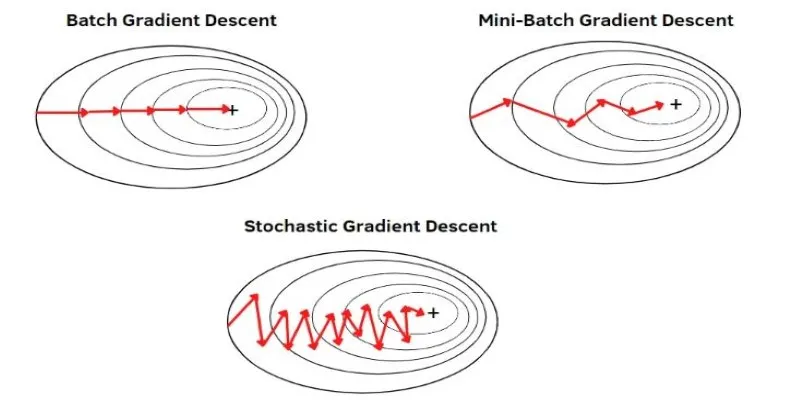
There are various gradients of gradient descent, each capable of dealing with different kinds of datasets and computational needs. The three most widely used types are batch gradient descent, stochastic gradient descent, and mini-batch gradient descent.
-
Batch Gradient Descent: This method calculates the gradient using the entire dataset before updating parameters. This ensures stability and smooth convergence but can be slow, especially with large datasets. The method requires significant memory, making it less suitable for high-dimensional data.
-
Stochastic Gradient Descent (SGD): This approach updates parameters after evaluating only a single data point. This makes learning much faster but also introduces randomness into the process. The trade-off is that while SGD can escape shallow local minima, it can also make erratic updates, leading to fluctuations in learning.
-
Mini-Batch Gradient Descent: This method strikes a balance between the two. Instead of using the entire dataset or a single point, it processes small batches of data at a time. This method reduces noise while still being computationally efficient. It is widely used in deep learning and large-scale machine learning applications.
Challenges and Improvements
Despite its effectiveness, gradient descent has some challenges. One major issue is getting stuck in local minima. In complex models, the cost function may have multiple valleys, and the algorithm can settle in a suboptimal one instead of reaching the lowest possible point. To mitigate this, techniques like momentum and adaptive learning rates are often used.
-
Momentum: This helps the algorithm maintain its direction even when encountering small fluctuations. Instead of adjusting parameters based solely on the current step, it also considers previous updates, allowing it to overcome small obstacles in the cost function.
-
Adaptive Learning Rate Methods: Techniques such as Adam and RMSprop modify the learning rate dynamically based on past gradients. These techniques help the model learn efficiently, especially when different parameters require different update rates.
Another challenge is choosing an appropriate learning rate. If it is too high, the model may never reach the optimal solution, bouncing around without converging. If it is too low, training can become excessively slow. Finding the right balance requires experimentation and sometimes fine-tuning.
Applications of Gradient Descent in Machine Learning
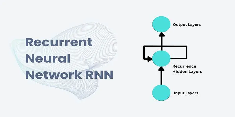
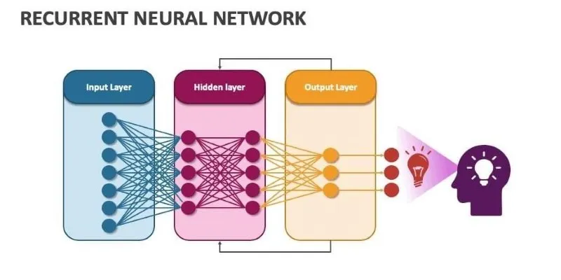
Gradient descent is widely used in various machine learning applications, playing a critical role in training models across different domains. In deep learning, neural networks rely on gradient descent to adjust their millions of parameters efficiently. Without it, optimizing complex architectures like convolutional and recurrent neural networks would be infeasible.

In natural language processing, models such as transformers and recurrent neural networks use gradient descent to learn patterns in text data. This allows them to generate human-like text, perform sentiment analysis, and improve machine translation. The ability to adjust weights based on gradients makes these models more accurate over time.
Gradient descent also powers recommendation systems, helping platforms like streaming services and e-commerce websites suggest relevant content to users. By minimizing errors in predicting user preferences, these systems become more effective at delivering personalized recommendations.
Beyond traditional machine learning, gradient descent is used in fields such as robotics, reinforcement learning, and scientific computing. Its ability to fine-tune models makes it indispensable for tasks ranging from self-driving cars to financial forecasting. The technique’s adaptability ensures its continued relevance as machine learning advances.
Conclusion
Gradient descent is the silent force behind machine learning, helping models refine their accuracy through continuous adjustments. Following the steepest downward path minimizes errors and fine-tunes predictions, making it indispensable in training everything from neural networks to recommendation systems. While challenges like local minima and learning rate selection exist, techniques like momentum and adaptive optimizers improve efficiency. Whether in deep learning or simpler models, gradient descent ensures machines learn effectively. Understanding this process isn’t just technical knowledge—it’s the key to building smarter, more precise AI systems that power real-world applications in every industry.