Artificial neural networks have shaped much of modern machine learning, and one of the most widely taught models is the multi-layer perceptron (MLP). Known for its ability to approximate complex patterns, the MLP remains a key building block in understanding how deep learning works.
To work effectively with MLPs, it helps to understand the mathematical notations used to describe them and how the trainable parameters — the weights and biases — are organized and optimized. This article explains these concepts clearly, focusing on how they fit together in the structure and training of an MLP.
Understanding the Structure and Notation of Multi-Layer Perceptrons
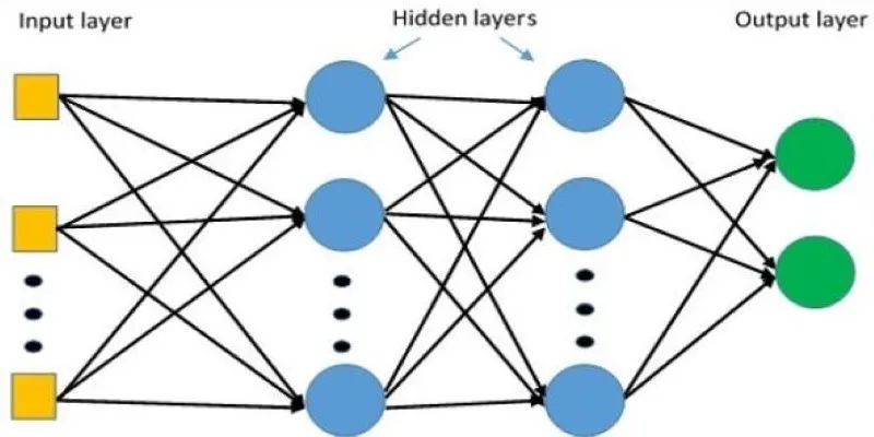
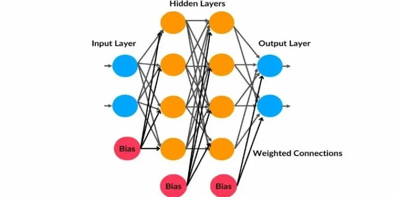
An MLP is a feedforward neural network composed of an input layer, one or more hidden layers, and an output layer. Each neuron in a layer receives inputs from all neurons in the previous layer, applies a weighted sum with a bias term, and passes the result through a nonlinear activation function. This continues layer by layer until the final output is produced.

The notation helps keep track of the transformations. Suppose an MLP has $L$ layers of weights (not counting the input layer), where each layer has $n^{[l]}$ neurons. The input vector $\mathbf{x}$ has $n^{[0]}$ features, equal to the size of the input layer.
For each layer we define:
- $\mathbf{W}^{[l]}$, the weight matrix of size $n^{[l]} \times n^{[l-1]}$, which connects the $j$-th neuron of the previous layer to the $k$-th neuron of the current layer.
- $\mathbf{b}^{[l]}$, the bias vector of size $n^{[l]}$, which shifts the activation thresholds.
- $\mathbf{z}^{[l]}$, the pre-activation vector: $\mathbf{z}^{[l]} = \mathbf{W}^{[l]}\mathbf{a}^{[l-1]} + \mathbf{b}^{[l]}$.
- $\mathbf{a}^{[l]}$, the activation output after applying a non-linear function to $\mathbf{z}^{[l]}$.
The first activation is simply the input $\mathbf{x}$. The activation function $\phi$ is often chosen as ReLU in hidden layers. The final layer’s activation depends on the task: softmax for classification or linear for regression. These notations concisely describe the forward pass through the network, making both implementation and analysis more manageable.
Counting and Interpreting Trainable Parameters
The strength of an MLP comes from its ability to learn the right values for its trainable parameters. These parameters are the weights and biases in each layer. Together, they determine how input signals are transformed as they pass through the network.
In layer $l$, the number of trainable weights equals the product $n^{[l]} \times n^{[l-1]}$, and the number of biases is $n^{[l]}$. Summing over all layers gives the total count of parameters in the network:
This total grows quickly as the number of layers and neurons increases, which is why MLPs with many layers or very wide layers can have millions of parameters. Each of these parameters is adjusted during training by an optimization algorithm such as stochastic gradient descent, which minimizes a chosen loss function by iteratively nudging the parameters in the right direction.
Understanding the parameter count also helps when diagnosing overfitting or underfitting. A model with too few parameters may struggle to capture the underlying pattern in the data. At the same time, a model with too many parameters relative to the data size may memorize the training data rather than generalizing to new examples.
Beyond just the count, it’s useful to appreciate what these parameters actually represent. Each weight can be thought of as encoding the strength and direction of the relationship between two neurons, while each bias shifts the activation threshold, allowing the neuron to fire even when its weighted inputs sum to zero. Together, weights and biases define a high-dimensional surface over which the optimizer searches for the lowest point — the combination of values that minimizes the loss.
Practical Considerations in Training MLPs
While the structure and parameters define the potential of an MLP, training determines how well that potential is realized. Because the number of parameters can be large, MLPs can be prone to challenges such as vanishing or exploding gradients during training, especially when using very deep architectures. Proper choice of activation functions, careful initialization of weights, and techniques like batch normalization or skip connections in deeper networks can help mitigate these issues.

Another practical aspect is regularization. Since MLPs often have many trainable parameters, they can overfit easily, especially when the amount of training data is limited. Regularization methods like dropout, weight decay, or early stopping help constrain the parameters to favor simpler models that generalize better.
The learning rate and batch size also influence how the parameters are updated during training. A learning rate that is too high might cause the parameters to oscillate without converging, while a very low learning rate could make training unnecessarily slow. Similarly, larger batch sizes provide more stable gradient estimates but require more memory.
Finally, the choice of loss function depends on the task at hand and defines what the MLP is optimizing. For regression tasks, mean squared error is common, while cross-entropy loss is preferred for classification tasks. This loss is computed at the output of the network, and its gradient with respect to each parameter is calculated using backpropagation, a systematic application of the chain rule that propagates gradients layer by layer backward through the network.
Conclusion
The multi-layer perceptron is one of the simplest neural network architectures, yet it remains highly relevant as a foundation for deeper and more specialized models. Its operation hinges on the interaction between its layers, described clearly through notations that track how inputs are transformed into outputs. The trainable parameters — weights and biases — define the flexibility of the model and are refined through training to fit the data. Understanding the structure, notations, and role of these parameters offers more than just a mathematical perspective; it gives insight into how neural networks learn and why their performance can vary. By keeping these concepts clear, it becomes easier to design, train, and troubleshoot MLPs in real-world machine learning tasks.
For further reading, consider exploring resources on deep learning techniques or practical machine learning applications.
 zfn9
zfn9


